本文探讨了缺失值插补算法的效果,强调选择合适的插补方法和评估指标的重要性。
原文标题:如何应对缺失值带来的分布变化?探索填充缺失值的最佳插补算法
原文作者:数据派THU
冷月清谈:
怜星夜思:
2、在不同的插补算法中,如何评估其效果?
3、如何应对缺失数据机制带来的挑战?
原文内容

来源:DeepHub IMBA本文约7800字,建议阅读13分钟
本文将探讨了缺失值插补的不同方法,并比较了它们在复原数据真实分布方面的效果。
数据
library(MASS) library(mice)set.seed(10)
n<-3000Xstar <- mvrnorm(n=n, mu=c(0,0), Sigma=matrix( c(1,0.7,0.7,1), nrow=2, byrow=T ))
colnames(Xstar) <- paste0(“X”,1:2)
Introduce missing mechanisms
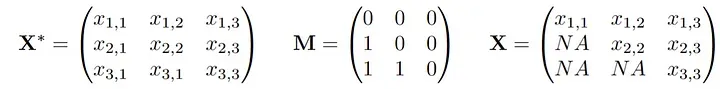
M<-matrix(0, ncol=ncol(Xstar), nrow=nrow(Xstar))
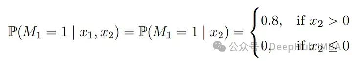
M[Xstar[,2] > 0, 1]<- sample(c(0,1), size=sum(Xstar[,2] > 0), replace=T, prob = c(1-0.8,0.8) )This gives rise to the observed dataset by masking X^* with M:
X<-Xstar
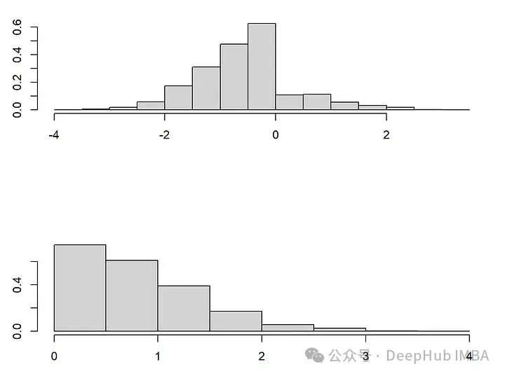
X[M==1] <- NAPlot the distribution shift
par(mfrow=c(2,1))
plot(Xstar[!is.na(X[,1]),1:2], xlab=“”, main=“”, ylab=“”, cex=0.8, col=“darkblue”, xlim=c(-4,4), ylim=c(-3,3))
plot(Xstar[is.na(X[,1]),1:2], xlab=“”, main=“”, ylab=“”, cex=0.8, col=“darkblue”, xlim=c(-4,4), ylim=c(-3,3))

插补是一个分布预测问题
## (0) Mean Imputation: This would correspond to "mean" in the mice R package ##1. Estimate the mean
meanX<-mean(X[!is.na(X[,1]),1])
2. Impute
meanimp<-X
meanimp[is.na(X[,1]),1] <-meanX(1) Regression Imputation: This would correspond to “norm.predict” in the mice R package
1. Estimate Regression
lmodelX1X2<-lm(X1~X2, data=as.data.frame(X[!is.na(X[,1]),]) )
2. Impute
impnormpredict<-X
impnormpredict[is.na(X[,1]),1] <-predict(lmodelX1X2, newdata= as.data.frame(X[is.na(X[,1]),]) )(2) Gaussian Imputation: This would correspond to “norm.nob” in the mice R package
1. Estimate Regression
#lmodelX1X2<-lm(X1~X2, X=as.data.frame(X[!is.na(X[,1]),]) )
(same as before)
2. Impute
impnorm<-X
meanx<-predict(lmodelX1X2, newdata= as.data.frame(X[is.na(X[,1]),]) )
var <- var(lmodelX1X2$residuals)
impnorm[is.na(X[,1]),1] <-rnorm(n=length(meanx), mean = meanx, sd=sqrt(var) )Plot the different imputations
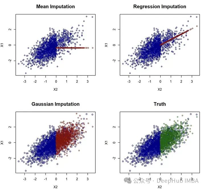
par(mfrow=c(2,2))
plot(meanimp[!is.na(X[,1]),c(“X2”,“X1”)], main=paste(“Mean Imputation”), cex=0.8, col=“darkblue”, cex.main=1.5)
points(meanimp[is.na(X[,1]),c(“X2”,“X1”)], col=“darkred”, cex=0.8 )plot(impnormpredict[!is.na(X[,1]),c(“X2”,“X1”)], main=paste(“Regression Imputation”), cex=0.8, col=“darkblue”, cex.main=1.5)
points(impnormpredict[is.na(X[,1]),c(“X2”,“X1”)], col=“darkred”, cex=0.8 )plot(impnorm[!is.na(X[,1]),c(“X2”,“X1”)], main=paste(“Gaussian Imputation”), col=“darkblue”, cex.main=1.5)
points(impnorm[is.na(X[,1]),c(“X2”,“X1”)], col=“darkred”, cex=0.8 )
#plot(Xstar[,c(“X2”,“X1”)], main=“Truth”, col=“darkblue”, cex.main=1.5)
plot(Xstar[!is.na(X[,1]),c(“X2”,“X1”)], main=“Truth”, col=“darkblue”, cex.main=1.5)
points(Xstar[is.na(X[,1]),c(“X2”,“X1”)], col=“darkgreen”, cex=0.8 )
## Regressing X_2 onto X_1mean imputation estimate
lm(X2~X1, data=data.frame(meanimp))$coefficients[“X1”]
beta= 0.61
regression imputation estimate
round(lm(X2~X1, data=data.frame(impnormpredict))$coefficients[“X1”],2)
beta= 0.90
Gaussian imputation estimate
round(lm(X2~X1, data=data.frame(impnorm))$coefficients[“X1”],2)
beta= 0.71
Truth imputation estimate
round(lm(X2~X1, data=data.frame(Xstar))$coefficients[“X1”],2)
beta= 0.71
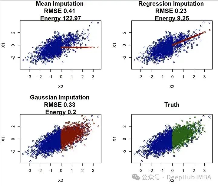
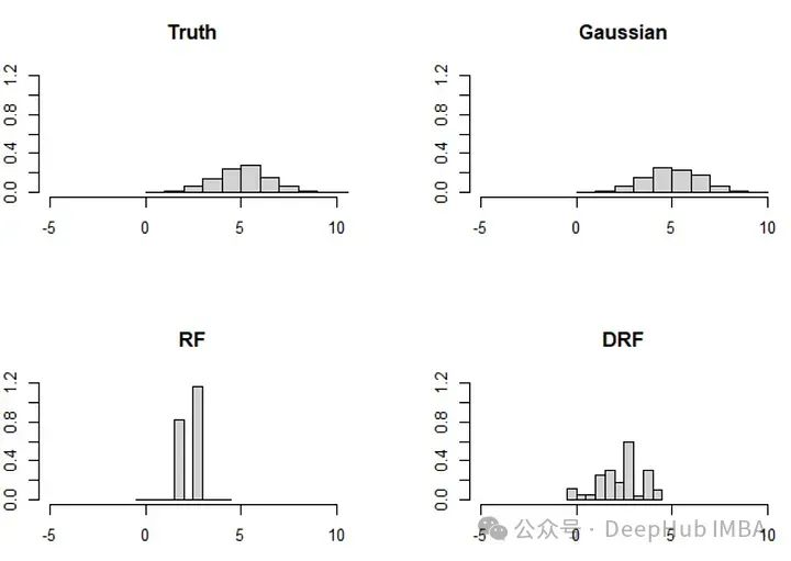
高斯插补的结果非常接近0.7(0.71),更重要的是,它非常接近使用完整(未观测)数据得到的估计!而均值插补低估了beta值,回归插补则高估了beta值。回归插补因为条件均值插补人为地增强了变量之间的关系,这将导致在科学和(数据科学)实践中估计出的效应被过高估计!
回归插补可能看起来过于简单,但是在机器学习和其他领域中非常常用的插补方法正是这样工作的。例如,knn插补和随机森林插补(即missForest)。特别是随机森林插补在几篇基准测试论文中受到赞扬和推荐,且应用非常广泛。missForest是在观测数据上拟合一个随机森林,然后简单地通过条件均值进行插补,使用它的结果将与回归插补非常相似,从而导致变量之间关系的人为强化和估计的偏差!
如何评估插补方法?

library(energy)Function to calculate the energy distance:
impX is the imputed data set
Xstar is the fully observed data set
Calculating the energy distance using the eqdist.e function of the energy package
energycalc <- function(impX, Xstar){
Note: eqdist.e calculates the energy statistics for a test, which is actually
= n^2/(2n)*energydistance(impX,Xstar), but we we are only interested in relative values
round(eqdist.e( rbind(Xstar,impX), c(nrow(Xstar), nrow(impX)) ),2)
}
par(mfrow=c(2,2))Same plots as before, but now with RMSE and energy distance
added
plot(meanimp[!is.na(X[,1]),c(“X2”,“X1”)], main=paste(“Mean Imputation”, “\nRMSE”, RMSEcalc(meanimp, Xstar), “\nEnergy”, energycalc(meanimp, Xstar)), cex=0.8, col=“darkblue”, cex.main=1.5)
points(meanimp[is.na(X[,1]),c(“X2”,“X1”)], col=“darkred”, cex=0.8 )plot(impnormpredict[!is.na(X[,1]),c(“X2”,“X1”)], main=paste(“Regression Imputation”,“\nRMSE”, RMSEcalc(impnormpredict, Xstar), “\nEnergy”, energycalc(impnormpredict, Xstar)), cex=0.8, col=“darkblue”, cex.main=1.5)
points(impnormpredict[is.na(X[,1]),c(“X2”,“X1”)], col=“darkred”, cex=0.8 )plot(impnorm[!is.na(X[,1]),c(“X2”,“X1”)], main=paste(“Gaussian Imputation”,“\nRMSE”, RMSEcalc(impnorm, Xstar), “\nEnergy”, energycalc(impnorm, Xstar)), col=“darkblue”, cex.main=1.5)
points(impnorm[is.na(X[,1]),c(“X2”,“X1”)], col=“darkred”, cex=0.8 )plot(Xstar[!is.na(X[,1]),c(“X2”,“X1”)], main=“Truth”, col=“darkblue”, cex.main=1.5)
points(Xstar[is.na(X[,1]),c(“X2”,“X1”)], col=“darkgreen”, cex=0.8 )
library(mice) source("Iscore.R")methods<-c(“mean”, #mice-mean
“norm.predict”, #mice-sample
“norm.nob”) # Gaussian ImputationWe first define functions that allow for imputation of the three methods:
imputationfuncs<-list()
imputationfuncs[[“mean”]] <- function(X,m){
1. Estimate the mean
meanX<-mean(X[!is.na(X[,1]),1])
2. Impute
meanimp<-X
meanimp[is.na(X[,1]),1] <-meanXres<-list()
for (l in 1:m){
res[[l]] <- meanimp
}return(res)
}
imputationfuncs[[“norm.predict”]] <- function(X,m){
1. Estimate Regression
lmodelX1X2<-lm(X1~., data=as.data.frame(X[!is.na(X[,1]),]) )
2. Impute
impnormpredict<-X
impnormpredict[is.na(X[,1]),1] <-predict(lmodelX1X2, newdata= as.data.frame(X[is.na(X[,1]),]) )res<-list()
for (l in 1:m){
res[[l]] <- impnormpredict
}return(res)
}
imputationfuncs[[“norm.nob”]] <- function(X,m){
1. Estimate Regression
lmodelX1X2<-lm(X1~., data=as.data.frame(X[!is.na(X[,1]),]) )
2. Impute
impnorm<-X
meanx<-predict(lmodelX1X2, newdata= as.data.frame(X[is.na(X[,1]),]) )
var <- var(lmodelX1X2$residuals)res<-list()
for (l in 1:m){
impnorm[is.na(X[,1]),1] <-rnorm(n=length(meanx), mean = meanx, sd=sqrt(var) )
res[[l]] <- impnorm
}return(res)
}
scoreslist <- Iscores_new(X,imputations=NULL, imputationfuncs=imputationfuncs, N=30)
scores<-do.call(cbind,lapply(scoreslist, function(x) x$score ))
names(scores)<-methods
scores[order(scores)]mean norm.predict norm.nob
-0.7455304 -0.5702136 -0.4220387
无需看到缺失数据的值,分数也能够识别分布,特别是当数据有两个以上的维度时。
随机缺失比你想象的更奇怪
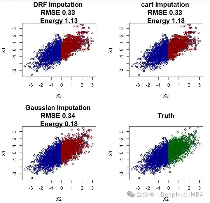
library(drf)mice-DRF
par(mfrow=c(2,2))
#Fit DRF
DRF <- drf(X=X[!is.na(X[,1]),2, drop=F], Y=X[!is.na(X[,1]),1, drop=F], num.trees=100)
impDRF<-XPredict weights for unobserved points
wx<-predict(DRF, newdata= X[is.na(X[,1]),2, drop=F] )$weights
impDRF[is.na(X[,1]),1] <-apply(wx,1,function(wxi) sample(X[!is.na(X[,1]),1, drop=F], size=1, replace=T, prob=wxi))plot(impDRF[!is.na(X[,1]),c(“X2”,“X1”)], main=paste(“DRF Imputation”, “\nRMSE”, RMSEcalc(impDRF, Xstar), “\nEnergy”, energycalc(impDRF, Xstar)), cex=0.8, col=“darkblue”, cex.main=1.5)
points(impDRF[is.na(X[,1]),c(“X2”,“X1”)], col=“darkred”, cex=0.8 )mice-cart##
impcart<-X
impcart[is.na(X[,1]),1] <-mice.impute.cart(X[,1], ry=!is.na(X[,1]), X[,2, drop=F], wy = NULL)plot(impDRF[!is.na(X[,1]),c(“X2”,“X1”)], main=paste(“cart Imputation”, “\nRMSE”, RMSEcalc(impcart, Xstar), “\nEnergy”, energycalc(impcart, Xstar)), cex=0.8, col=“darkblue”, cex.main=1.5)
points(impDRF[is.na(X[,1]),c(“X2”,“X1”)], col=“darkred”, cex=0.8 )plot(impnorm[!is.na(X[,1]),c(“X2”,“X1”)], main=paste(“Gaussian Imputation”,“\nRMSE”, RMSEcalc(impnorm, Xstar), “\nEnergy”, energycalc(impnorm, Xstar)), col=“darkblue”, cex.main=1.5)
points(impnorm[is.na(X[,1]),c(“X2”,“X1”)], col=“darkred”, cex=0.8 )
总结
最后本文引用的论文:
What Is a Good Imputation Under MAR Missingness? [1]
https://hal.science/hal-04521894
