本文探讨多项式朴素贝叶斯分类器的原理与应用,尤其在文本分类中的实现方法。
原文标题:多项式朴素贝叶斯分类器
原文作者:数据派THU
冷月清谈:
怜星夜思:
2、使用平滑技巧处理未出现特征有什么重要性?
3、对数空间中的计算方法有什么优势?
原文内容

来源:Deephub Imba本文约6500字,建议阅读10分钟我们介绍多项式朴素贝叶斯分类器是如何工作的,然后使用scikit-learn作为实际工作的示例来介绍如何使用。

多项分布


loaded_dice_probs = [1/6, 1/4, 1/4, 1/6, 1/12, 1/12]
dice_faces = [1, 2, 3, 4, 5, 6]
n_try = 100
# Sample the distribution
sampled_loaded_dice = np.random.multinomial(n_try, loaded_dice_probs)
sampled_loaded_dice
#--> array([17, 26, 21, 18, 8, 10])


分类问题


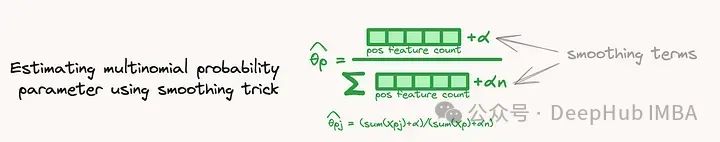
使用平滑技巧估计多项参数


在对数空间计算预测,避免数值下溢


import numpy as np
J = 10000
nsamples = 300
X = np.random.choice(np.arange(1, 50), size=(nsamples,J))
# split into train and test (test has only 1 sample)
X_train, X_test = X[:-1], X[-1]
# estimate the distribution probabilities
feature_probs = X_train.sum(axis=0)/ X_train.sum()
print(feature_probs)
# [9.53780825e-05 1.05477725e-04 1.03631698e-04 … 1.07925718e-04
# 1.09517582e-04 9.51506733e-05]
# compute the probability for the test sample
print(feature_probs ** X_test)
print(np.prod(feature_probs ** X_test))
[1.37037886e-169 2.34731879e-064 5.34752484e-188 ... 1.84077019e-032
1.72545280e-024 4.29538125e-069]
0.0


Python示例

import numpy as np import pandas as pd import matplotlib.pyplot as plt import seaborn as sns from sklearn.feature_extraction.text import CountVectorizer from sklearn.model_selection import train_test_split from sklearn.naive_bayes import MultinomialNBDefine the vocabulary
vocabulary = [‘good’, ‘bad’, ‘excellent’, ‘poor’, ‘great’, ‘terrible’, ‘awesome’, ‘awful’, ‘fantastic’, ‘horrible’]
here the learned vocabulary is set from the begining
it is usually created with the dataset but for this we assume it is limited to this list
Define probabilities for positive distribution
note that probabilities for “bad” words are not 0, so they might appear in positive docs, and vice versa
also, normalize probabilities to sum to
positive_probs = np.array([0.3, 0.1, 0.5, 0.1, 0.4, 0.1, 0.6, 0.1, 0.5, 0.1])
negative_probs = np.array([0.1, 0.3, 0.1, 0.5, 0.1, 0.4, 0.1, 0.6, 0.1, 0.5])
positive_probs /= positive_probs.sum()
negative_probs /= negative_probs.sum()Let’s plot each distribution
df = pd.DataFrame({‘neg’: negative_probs, ‘pos’: positive_probs},index=vocabulary)
df_melted = df.reset_index(names=‘word’).melt(id_vars=‘word’, value_vars=[‘pos’, ‘neg’], var_name=“class”, value_name=“prob.”)
g = sns.catplot(df_melted, y=“prob.”, hue=“class”, x=‘word’, kind=‘bar’)
g.ax.set_xticklabels(g.ax.get_xticklabels(), rotation=90, ha=‘center’, va=‘top’)
g.ax.set_title(‘True distrbutions’)


# Generate random documents for each class # create 1000 positive reviews and 1000 negative reviews : our dataset is balanced # the length (=number of words=sum of each row) may vary between 5 and 15 words) # note that the vocabulary of each review (=number of distinct word) may be different n_samples = 1000 positive_docs = [' '.join(np.random.choice(vocabulary, size=np.random.randint(5, 15), p=positive_probs)) for _ in range(n_samples)] negative_docs = [' '.join(np.random.choice(vocabulary, size=np.random.randint(5, 15), p=negative_probs)) for _ in range(n_samples)]Create labels
labels_positive = np.ones(n_samples, dtype=int)
labels_negative = np.zeros(n_samples, dtype=int)Combine documents and labels
documents = np.concatenate([positive_docs, negative_docs])
labels = np.concatenate([labels_positive, labels_negative])
plt.figure()
sns.heatmap(CountVectorizer(vocabulary=vocabulary).fit_transform(documents).toarray(), xticklabels=vocabulary, cbar_kws={‘label’:‘word count’})#, cmap=“copper”)

X_train, X_test, y_train, y_test = train_test_split(documents, labels, test_size=0.2, random_state=42, shuffle=True)Create a CountVectorizer to convert documents into a matrix of token counts
vectorizer = CountVectorizer(vocabulary=vocabulary)
Fit and transform the training data
X_train_counts = vectorizer.fit_transform(X_train)
Train a multinomial naive Bayes classifier
classifier = MultinomialNB(alpha=0) # notice I use alpha=0 here because I control the dataset and know there are no “empty” feature
classifier.fit(X_train_counts, y_train)
for class_, count_, feature_count_ in zip(classifier.classes_, classifier.class_count_, classifier.feature_count_):
print(“For class”, class_, "there were ", count_, “instance in the dataset. For those samples, the total counts for each word is”, feature_count_)estimate distribution parametsers ourselves from scikit-learn stored attributes
thetas = (classifier.feature_count_.T / classifier.feature_count_.sum(axis=1)).T
print(thetas)sort by class
X_train_pos = X_train_counts[y_train==0]
X_train_neg = X_train_counts[y_train==1]
print(X_train_pos.sum(axis=0)/X_train_pos.sum(), X_train_neg.sum(axis=0)/X_train_neg.sum())
df = pd.DataFrame({‘neg’: thetas[0], ‘pos’: thetas[1]}, index=vocabulary)
df_melted = df.reset_index(names=‘word’).melt(id_vars=‘word’, value_vars=[‘pos’, ‘neg’], var_name=“class”, value_name=“prob.”)
g = sns.catplot(df_melted, y=“prob.”, hue=“class”, x=‘word’, kind=‘bar’)
g.ax.set_xticklabels(g.ax.get_xticklabels(), rotation=90, ha=‘center’, va=‘top’)
g.ax.set_title(‘Learned distrbutions’)
For class 0 there were 799.0 instance in the dataset. For those samples, the total counts for each word is [ 258. 815. 256. 1274. 294. 1134. 296. 1618. 264. 1402.]
For class 1 there were 801.0 instance in the dataset. For those samples, the total counts for each word is [ 827. 277. 1306. 281. 1121. 293. 1618. 228. 1344. 244.]
[[0.03389831 0.10708186 0.03363553 0.1673893 0.0386283 0.14899488
0.03889108 0.21258705 0.03468664 0.18420707]
[0.10969625 0.03674227 0.17323252 0.03727285 0.14869346 0.03886457
0.21461732 0.03024274 0.17827298 0.03236504]]
[[0.03389831 0.10708186 0.03363553 0.1673893 0.0386283 0.14899488
0.03889108 0.21258705 0.03468664 0.18420707]]
[[0.10969625 0.03674227 0.17323252 0.03727285 0.14869346 0.03886457
0.21461732 0.03024274 0.17827298 0.03236504]]

x_new = vectorizer.transform(X_test)[0].toarray()[0]
x_normed = x_new / x_new.sum()
df = pd.DataFrame({‘neg’: thetas[1], ‘pos’: thetas[0], ‘new’:x_normed}, index=vocabulary)

df_melted = df.reset_index(names=‘word’).melt(id_vars=‘word’, value_vars=[‘pos’, ‘new’, ‘neg’], var_name=“class”, value_name=‘prob.’)

g = sns.catplot(df_melted, y=“prob.”, hue=“class”, x=‘word’, kind=‘bar’)

g.ax.set_xticklabels(g.ax.get_xticklabels(), rotation=90, ha=‘center’, va=‘top’)

g.ax.set_title(‘Learned distrbutions along with new sample to predict’)
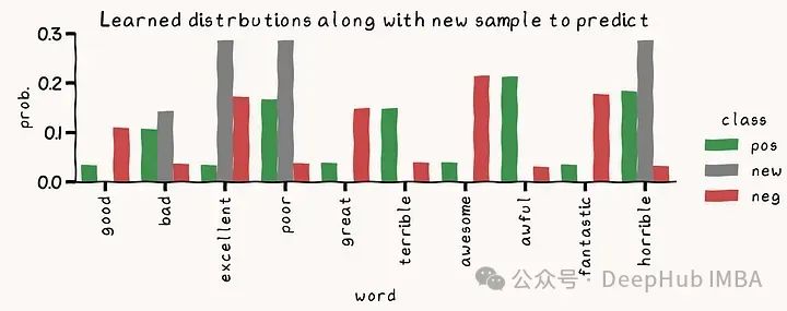
classifier.predict([x_new])
#--> array([0])
x_new = [vectorizer.transform(X_test)[0].toarray()[0]]class log prior
print(classifier.class_log_prior_)
print(np.log(classifier.class_count_/classifier.class_count_.sum()))feature log
print(classifier.feature_log_prob_)
print(np.log(classifier.feature_count_.T / classifier.feature_count_.sum(axis=1)).T)final log likelihood
print(classifier.predict_joint_log_proba(x_new))
jll = np.dot(x_new, np.log(classifier.feature_count_.T / classifier.feature_count_.sum(axis=1))) + np.log(classifier.class_count_/classifier.class_count_.sum())
print(jll)log prob.
print(classifier.predict_log_proba(x_new))
from scipy.special import logsumexp
log_prob_x = logsumexp(jll, axis=1)
print(jll - np.atleast_2d(log_prob_x).T)last 3 lines are equivalent to normalizing the sum of probability in ‘not-log-space’: x_ = x_ / x_.sum()
final prob
print(classifier.predict_proba(x_new))
print(np.exp(jll - np.atleast_2d(log_prob_x).T))
[-0.69439796 -0.69189796]
[-0.69439796 -0.69189796]
[[-3.38439026 -2.23416174 -3.3921724 -1.78743301 -3.25377008 -1.90384336
-3.24699039 -1.54840375 -3.36140075 -1.69169478]
[-2.21004013 -3.30382732 -1.75312052 -3.28949016 -1.9058684 -3.24767222
-1.53889873 -3.4984992 -1.72443931 -3.4306766 ]]
[[-3.38439026 -2.23416174 -3.3921724 -1.78743301 -3.25377008 -1.90384336
-3.24699039 -1.54840375 -3.36140075 -1.69169478]
[-2.21004013 -3.30382732 -1.75312052 -3.28949016 -1.9058684 -3.24767222
-1.53889873 -3.4984992 -1.72443931 -3.4306766 ]]
[[-16.67116009 -20.94229983]]
[[-16.67116009 -20.94229983]]
[[-0.01386923 -4.28500897]]
[[-0.01386923 -4.28500897]]
[[0.9862265 0.0137735]]
[[0.9862265 0.0137735]]
总结
多项分布是一种重要的概率分布,适用于描述多类别、多次试验的情况,是概率论和统计学中的基础之一。它表示实验可以有N个不同的输出,重复M次。可以把它看作投掷硬币的二项分布的概括,就像反复计算掷骰子的每面一样。多项式朴素贝叶斯分类器的总体思想与高斯朴素贝叶斯分类器非常相似,只是在拟合和预测计算上有所不同。为了学习每个类别的多项概率参数,可以简单地将训练集沿特征求和,并将结果除以该向量的和。这提供了对概率的估计。使用一个平滑的技巧可以处理在训练中未出现的特征。为了预测新样本的类别,则需要使用多项分布的概率质量函数,并在“对数空间”中计算所有概率,以避免下溢和计算机无法处理的小数字。
多项分布在实际中有广泛的应用,特别是在以下领域:
-
自然语言处理中的文本分类、主题建模等。
-
生物统计学中的多样性指数的计算。
-
计数数据的建模,如调查数据、市场调查等。
-
假设检验,用于检验多类别随机变量的比例是否满足某种期望。
编辑:王菁
校对:林亦霖
