原文标题:GitHub 爆款项目:详解 llama3 实现,已获 8.7k Star!
原文作者:机器学习算法与Python学习
冷月清谈:
怜星夜思:
2、在使用 llama3 之前,需要进行哪些准备工作?
3、如何评价 llama3 的易用性?
原文内容

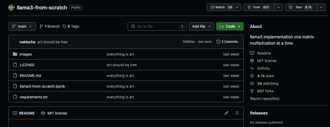
项目地址:https://github.com/naklecha/llama3-from-scratch
项目地址:https://github.com/naklecha/llama3-from-scratch
项目地址:https://github.com/naklecha/llama3-from-scratch

from pathlib import Path
import tiktoken
from tiktoken.load import load_tiktoken_bpe
import torch
import json
import matplotlib.pyplot as plt
tokenizer_path = "Meta-Llama-3-8B/tokenizer.model"
special_tokens = [
"<|begin_of_text|>",
"<|end_of_text|>",
"<|reserved_special_token_0|>",
"<|reserved_special_token_1|>",
"<|reserved_special_token_2|>",
"<|reserved_special_token_3|>",
"<|start_header_id|>",
"<|end_header_id|>",
"<|reserved_special_token_4|>",
"<|eot_id|>",  # end of turn
] + [f"<|reserved_special_token_{i}|>" for i in range (5, 256 - 5)] mergeable_ranks = load_tiktoken_bpe (tokenizer_path) tokenizer = tiktoken.Encoding (
name=Path (tokenizer_path).name,
pat_str=r"(?i:'s|'t|'re|'ve|'m|'ll|'d)|[^\r\n\p {L}\p {N}]?\p {L}+|\p {N}{1,3}| ?[^\s\p {L}\p {N}]+[\r\n]*|\s*[\r\n]+|\s+(?!\S)|\s+",
mergeable_ranks=mergeable_ranks,
special_tokens={token: len (mergeable_ranks) + i for i, token in enumerate (special_tokens)},
)
tokenizer.decode (tokenizer.encode ("hello world!"))
'hello world!'
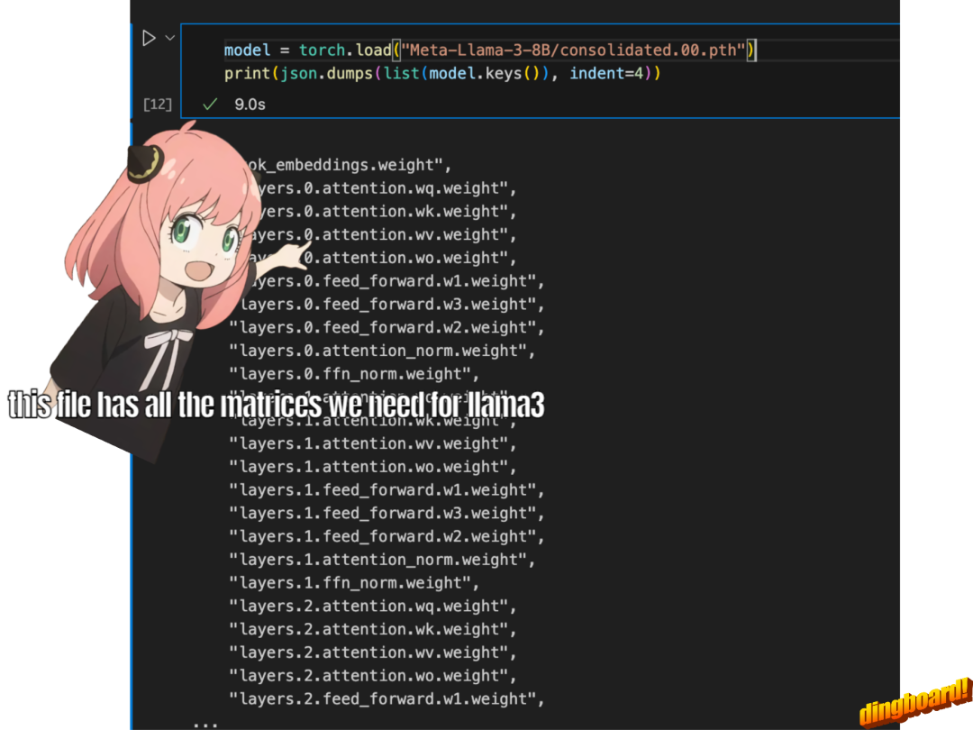
model = torch.load ("Meta-Llama-3-8B/consolidated.00.pth")
print (json.dumps (list (model.keys ())[:20], indent=4))
[
"tok_embeddings.weight",
"layers.0.attention.wq.weight",
"layers.0.attention.wk.weight",
"layers.0.attention.wv.weight",
"layers.0.attention.wo.weight",
"layers.0.feed_forward.w1.weight",
"layers.0.feed_forward.w3.weight",
"layers.0.feed_forward.w2.weight",
"layers.0.attention_norm.weight",
"layers.0.ffn_norm.weight",
"layers.1.attention.wq.weight",
"layers.1.attention.wk.weight",
"layers.1.attention.wv.weight",
"layers.1.attention.wo.weight",
"layers.1.feed_forward.w1.weight",
"layers.1.feed_forward.w3.weight",
"layers.1.feed_forward.w2.weight",
"layers.1.attention_norm.weight",
"layers.1.ffn_norm.weight",
"layers.2.attention.wq.weight"
]
with open ("Meta-Llama-3-8B/params.json", "r") as f:
config = json.load (f)
config
{'dim': 4096,
'n_layers': 32,
'n_heads': 32,
'n_kv_heads': 8,
'vocab_size': 128256,
'multiple_of': 1024,
'ffn_dim_multiplier': 1.3,
'norm_eps': 1e-05,
'rope_theta': 500000.0}
-
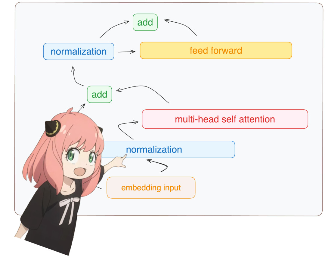
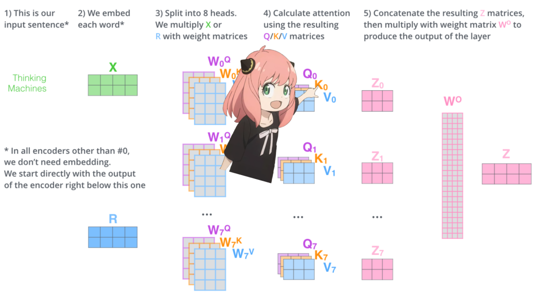
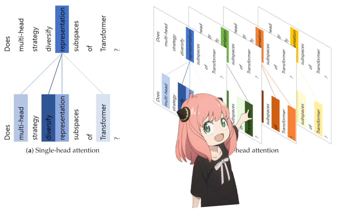
模型有 32 个 transformer 层;
-
每个多头注意力块有 32 个头。
dim = config ["dim"]
n_layers = config ["n_layers"]
n_heads = config ["n_heads"]
n_kv_heads = config ["n_kv_heads"]
vocab_size = config ["vocab_size"]
multiple_of = config ["multiple_of"]
ffn_dim_multiplier = config ["ffn_dim_multiplier"]
norm_eps = config ["norm_eps"]
rope_theta = torch.tensor (config ["rope_theta"])
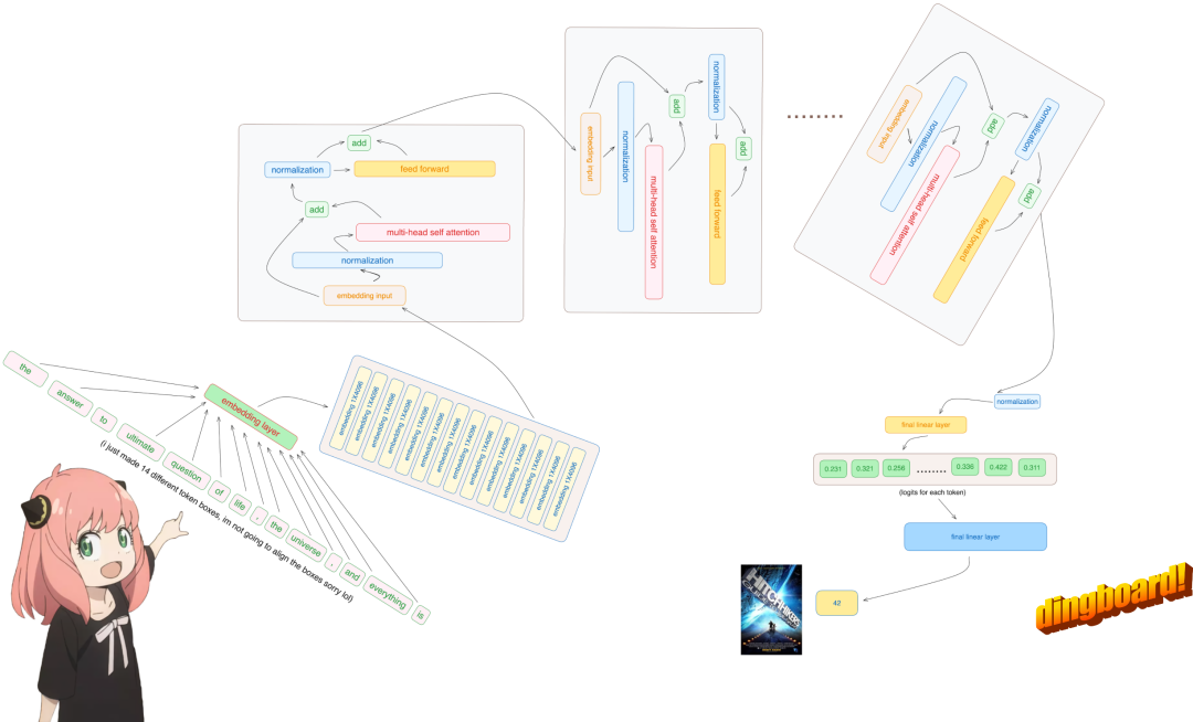
prompt = "the answer to the ultimate question of life, the universe, and everything is"
tokens = [128000] + tokenizer.encode (prompt)
print (tokens)
tokens = torch.tensor (tokens)
prompt_split_as_tokens = [tokenizer.decode ([token.item ()]) for token in tokens]
print (prompt_split_as_tokens)
[128000, 1820, 4320, 311, 279, 17139, 3488, 315, 2324, 11, 279, 15861, 11, 323, 4395, 374, 220]
['<|begin_of_text|>', 'the', ' answer', ' to', ' the', ' ultimate', ' question', ' of', ' life', ',', ' the', ' universe', ',', ' and', ' everything', ' is', ' ']

embedding_layer = torch.nn.Embedding (vocab_size, dim)
embedding_layer.weight.data.copy_(model ["tok_embeddings.weight"])
token_embeddings_unnormalized = embedding_layer (tokens).to (torch.bfloat16)
token_embeddings_unnormalized.shape
torch.Size ([17, 4096])

# def rms_norm (tensor, norm_weights):
#     rms = (tensor.pow (2).mean (-1, keepdim=True) + norm_eps)**0.5
#     return tensor * (norm_weights /rms)
def rms_norm (tensor, norm_weights):
return (tensor * torch.rsqrt (tensor.pow (2).mean (-1, keepdim=True) + norm_eps)) * norm_weights
token_embeddings = rms_norm (token_embeddings_unnormalized, model ["layers.0.attention_norm.weight"])
token_embeddings.shape
torch.Size ([17, 4096])
print (
model ["layers.0.attention.wq.weight"].shape,
model ["layers.0.attention.wk.weight"].shape,
model ["layers.0.attention.wv.weight"].shape,
model ["layers.0.attention.wo.weight"].shape
)
torch.Size ([4096, 4096]) torch.Size ([1024, 4096]) torch.Size ([1024, 4096]) torch.Size ([4096, 4096])
q_layer0 = model ["layers.0.attention.wq.weight"]
head_dim = q_layer0.shape [0] //n_heads
q_layer0 = q_layer0.view (n_heads, head_dim, dim)
q_layer0.shape
torch.Size ([32, 128, 4096])
q_layer0_head0 = q_layer0 [0]
q_layer0_head0.shape
torch.Size ([128, 4096])
q_per_token = torch.matmul (token_embeddings, q_layer0_head0.T)
q_per_token.shape
torch.Size ([17, 128])
q_per_token_split_into_pairs = q_per_token.float ().view (q_per_token.shape [0], -1, 2)
q_per_token_split_into_pairs.shape
torch.Size ([17, 64, 2])
zero_to_one_split_into_64_parts = torch.tensor (range (64))/64
zero_to_one_split_into_64_parts
tensor ([0.0000, 0.0156, 0.0312, 0.0469, 0.0625, 0.0781, 0.0938, 0.1094, 0.1250,
0.1406, 0.1562, 0.1719, 0.1875, 0.2031, 0.2188, 0.2344, 0.2500, 0.2656,
0.2812, 0.2969, 0.3125, 0.3281, 0.3438, 0.3594, 0.3750, 0.3906, 0.4062,
0.4219, 0.4375, 0.4531, 0.4688, 0.4844, 0.5000, 0.5156, 0.5312, 0.5469,
0.5625, 0.5781, 0.5938, 0.6094, 0.6250, 0.6406, 0.6562, 0.6719, 0.6875,
0.7031, 0.7188, 0.7344, 0.7500, 0.7656, 0.7812, 0.7969, 0.8125, 0.8281,
0.8438, 0.8594, 0.8750, 0.8906, 0.9062, 0.9219, 0.9375, 0.9531, 0.9688,
0.9844])
freqs = 1.0 / (rope_theta ** zero_to_one_split_into_64_parts)
freqs
tensor ([1.0000e+00, 8.1462e-01, 6.6360e-01, 5.4058e-01, 4.4037e-01, 3.5873e-01,
2.9223e-01, 2.3805e-01, 1.9392e-01, 1.5797e-01, 1.2869e-01, 1.0483e-01,
8.5397e-02, 6.9566e-02, 5.6670e-02, 4.6164e-02, 3.7606e-02, 3.0635e-02,
2.4955e-02, 2.0329e-02, 1.6560e-02, 1.3490e-02, 1.0990e-02, 8.9523e-03,
7.2927e-03, 5.9407e-03, 4.8394e-03, 3.9423e-03, 3.2114e-03, 2.6161e-03,
2.1311e-03, 1.7360e-03, 1.4142e-03, 1.1520e-03, 9.3847e-04, 7.6450e-04,
6.2277e-04, 5.0732e-04, 4.1327e-04, 3.3666e-04, 2.7425e-04, 2.2341e-04,
1.8199e-04, 1.4825e-04, 1.2077e-04, 9.8381e-05, 8.0143e-05, 6.5286e-05,
5.3183e-05, 4.3324e-05, 3.5292e-05, 2.8750e-05, 2.3420e-05, 1.9078e-05,
1.5542e-05, 1.2660e-05, 1.0313e-05, 8.4015e-06, 6.8440e-06, 5.5752e-06,
4.5417e-06, 3.6997e-06, 3.0139e-06, 2.4551e-06])
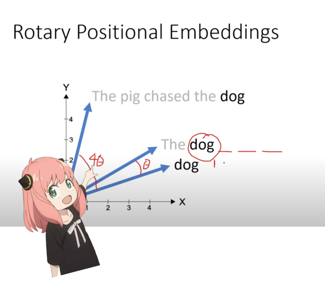
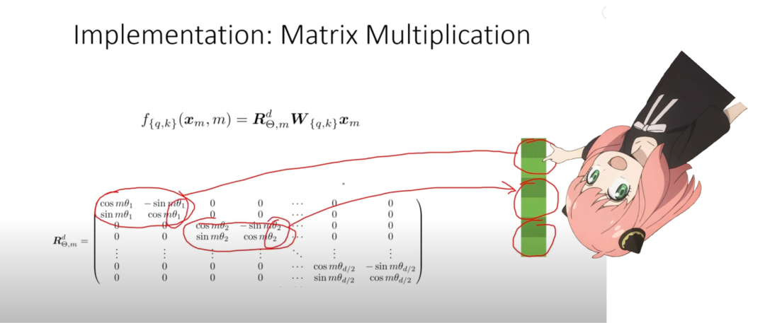
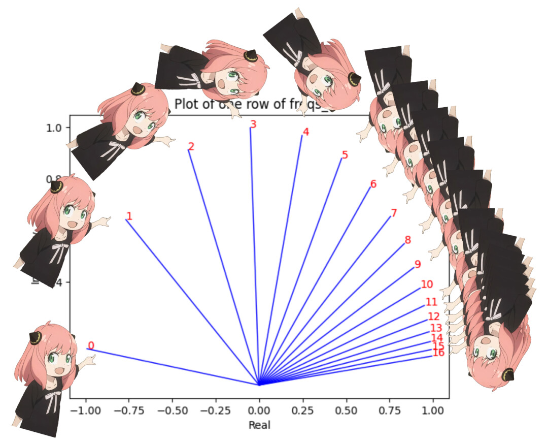
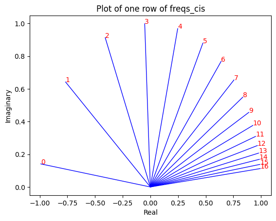
freqs_for_each_token = torch.outer (torch.arange (17), freqs)
freqs_cis = torch.polar (torch.ones_like (freqs_for_each_token), freqs_for_each_token)
freqs_cis.shape
# viewing tjhe third row of freqs_cis
value = freqs_cis [3]
plt.figure ()
for i, element in enumerate (value [:17]):
plt.plot ([0, element.real], [0, element.imag], color='blue', linewidth=1, label=f"Index: {i}")
plt.annotate (f"{i}", xy=(element.real, element.imag), color='red')
plt.xlabel ('Real')
plt.ylabel ('Imaginary')
plt.title ('Plot of one row of freqs_cis')
plt.show ()
q_per_token_as_complex_numbers = torch.view_as_complex (q_per_token_split_into_pairs)
q_per_token_as_complex_numbers.shape
torch.Size ([17, 64])
q_per_token_as_complex_numbers_rotated = q_per_token_as_complex_numbers * freqs_cis
q_per_token_as_complex_numbers_rotated.shape
torch.Size ([17, 64])
q_per_token_split_into_pairs_rotated = torch.view_as_real (q_per_token_as_complex_numbers_rotated)
q_per_token_split_into_pairs_rotated.shape
torch.Size ([17, 64, 2])
q_per_token_rotated = q_per_token_split_into_pairs_rotated.view (q_per_token.shape)
q_per_token_rotated.shape
torch.Size ([17, 128])
k_layer0 = model ["layers.0.attention.wk.weight"]
k_layer0 = k_layer0.view (n_kv_heads, k_layer0.shape [0] //n_kv_heads, dim)
k_layer0.shape
torch.Size ([8, 128, 4096])
k_layer0_head0 = k_layer0 [0]
k_layer0_head0.shape
torch.Size ([128, 4096])
k_per_token = torch.matmul (token_embeddings, k_layer0_head0.T)
k_per_token.shape
torch.Size ([17, 128])
k_per_token_split_into_pairs = k_per_token.float ().view (k_per_token.shape [0], -1, 2)
k_per_token_split_into_pairs.shape
torch.Size ([17, 64, 2])
k_per_token_as_complex_numbers = torch.view_as_complex (k_per_token_split_into_pairs)
k_per_token_as_complex_numbers.shape
torch.Size ([17, 64])
k_per_token_split_into_pairs_rotated = torch.view_as_real (k_per_token_as_complex_numbers * freqs_cis)
k_per_token_split_into_pairs_rotated.shape
torch.Size ([17, 64, 2])
k_per_token_rotated = k_per_token_split_into_pairs_rotated.view (k_per_token.shape)
k_per_token_rotated.shape
torch.Size ([17, 128])
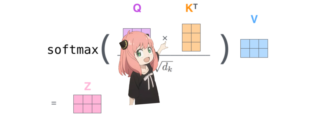
qk_per_token = torch.matmul (q_per_token_rotated, k_per_token_rotated.T)/(head_dim)**0.5
qk_per_token.shape
torch.Size ([17, 17])
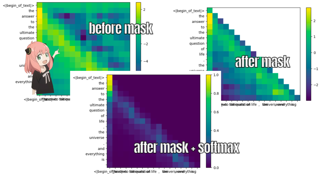
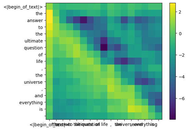
def display_qk_heatmap (qk_per_token):
_, ax = plt.subplots ()
im = ax.imshow (qk_per_token.to (float).detach (), cmap='viridis')
ax.set_xticks (range (len (prompt_split_as_tokens)))
ax.set_yticks (range (len (prompt_split_as_tokens)))
ax.set_xticklabels (prompt_split_as_tokens)
ax.set_yticklabels (prompt_split_as_tokens)
ax.figure.colorbar (im, ax=ax)
display_qk_heatmap (qk_per_token)
mask = torch.full ((len (tokens), len (tokens)), float ("-inf"), device=tokens.device) mask = torch.triu (mask, diagonal=1) mask
tensor ([[0., -inf, -inf, -inf, -inf, -inf, -inf, -inf, -inf, -inf, -inf, -inf, -inf, -inf, -inf, -inf, -inf],
[0., 0., -inf, -inf, -inf, -inf, -inf, -inf, -inf, -inf, -inf, -inf, -inf, -inf, -inf, -inf, -inf],
[0., 0., 0., -inf, -inf, -inf, -inf, -inf, -inf, -inf, -inf, -inf, -inf, -inf, -inf, -inf, -inf],
[0., 0., 0., 0., -inf, -inf, -inf, -inf, -inf, -inf, -inf, -inf, -inf, -inf, -inf, -inf, -inf],
[0., 0., 0., 0., 0., -inf, -inf, -inf, -inf, -inf, -inf, -inf, -inf, -inf, -inf, -inf, -inf],
[0., 0., 0., 0., 0., 0., -inf, -inf, -inf, -inf, -inf, -inf, -inf, -inf, -inf, -inf, -inf],
[0., 0., 0., 0., 0., 0., 0., -inf, -inf, -inf, -inf, -inf, -inf, -inf, -inf, -inf, -inf],
[0., 0., 0., 0., 0., 0., 0., 0., -inf, -inf, -inf, -inf, -inf, -inf, -inf, -inf, -inf],
[0., 0., 0., 0., 0., 0., 0., 0., 0., -inf, -inf, -inf, -inf, -inf, -inf, -inf, -inf],
[0., 0., 0., 0., 0., 0., 0., 0., 0., 0., -inf, -inf, -inf, -inf, -inf, -inf, -inf],
[0., 0., 0., 0., 0., 0., 0., 0., 0., 0., 0., -inf, -inf, -inf, -inf, -inf, -inf],
[0., 0., 0., 0., 0., 0., 0., 0., 0., 0., 0., 0., -inf, -inf, -inf, -inf, -inf],
[0., 0., 0., 0., 0., 0., 0., 0., 0., 0., 0., 0., 0., -inf, -inf, -inf, -inf],
[0., 0., 0., 0., 0., 0., 0., 0., 0., 0., 0., 0., 0., 0., -inf, -inf, -inf],
[0., 0., 0., 0., 0., 0., 0., 0., 0., 0., 0., 0., 0., 0., 0., -inf, -inf],
[0., 0., 0., 0., 0., 0., 0., 0., 0., 0., 0., 0., 0., 0., 0., 0., -inf],
[0., 0., 0., 0., 0., 0., 0., 0., 0., 0., 0., 0., 0., 0., 0., 0., 0.]])
qk_per_token_after_masking = qk_per_token + mask
display_qk_heatmap (qk_per_token_after_masking)
qk_per_token_after_masking_after_softmax = torch.nn.functional.softmax (qk_per_token_after_masking, dim=1).to (torch.bfloat16) display_qk_heatmap (qk_per_token_after_masking_after_softmax)
-
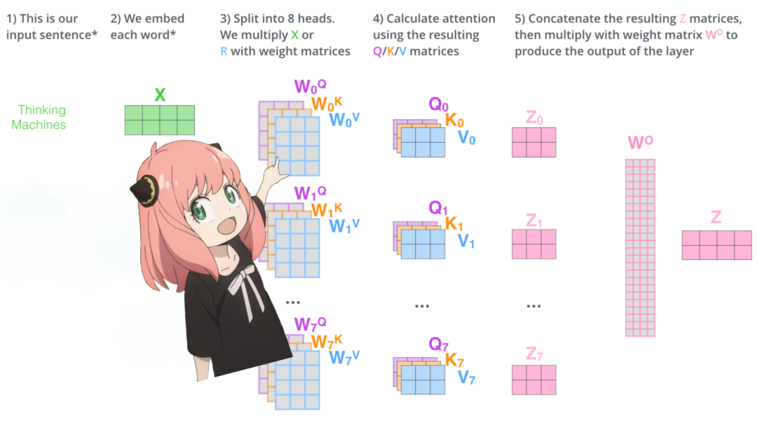
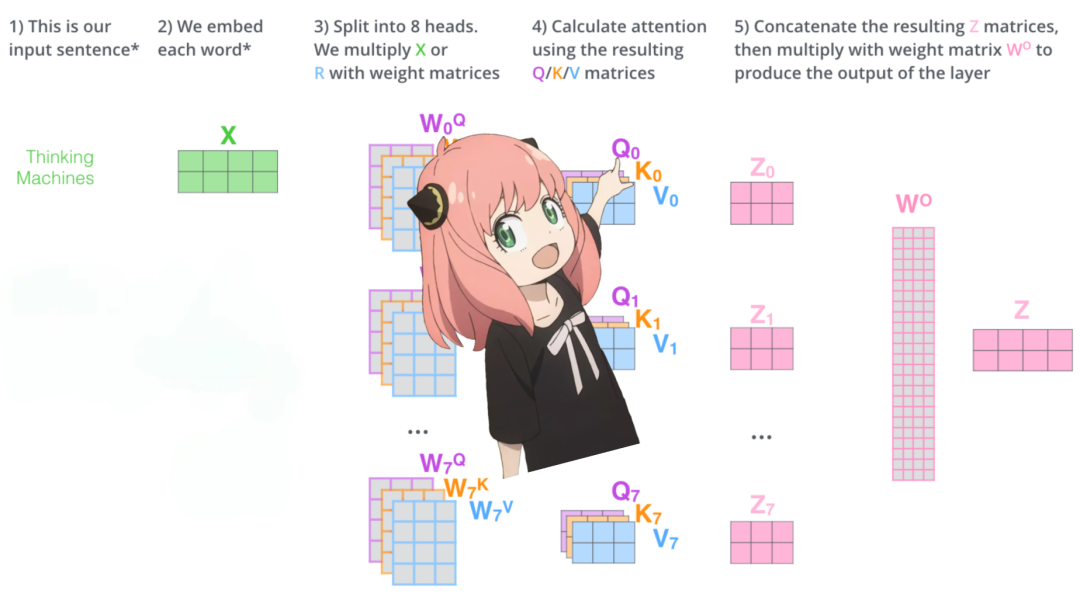
就像键一样,值权重也在 4 个注意力头之间共享(以节省计算量)
-
结果,下面的值权重矩阵形状为 [8x128x4096]
v_layer0 = model ["layers.0.attention.wv.weight"] v_layer0 = v_layer0.view (n_kv_heads, v_layer0.shape [0] //n_kv_heads, dim) v_layer0.shape
torch.Size ([8, 128, 4096])
v_layer0_head0 = v_layer0 [0] v_layer0_head0.shape
torch.Size ([128, 4096])
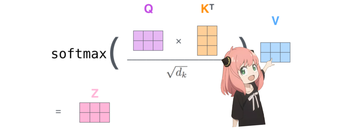
v_per_token = torch.matmul (token_embeddings, v_layer0_head0.T)v_per_token.shape
torch.Size ([17, 128])
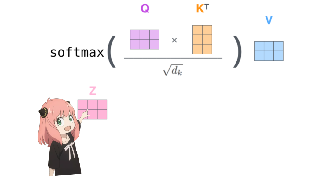
qkv_attention = torch.matmul (qk_per_token_after_masking_after_softmax, v_per_token) qkv_attention.shape
torch.Size ([17, 128])
qkv_attention_store = [] for head in range (n_heads): q_layer0_head = q_layer0 [head] k_layer0_head = k_layer0 [head//4] # key weights are shared across 4 heads v_layer0_head = v_layer0 [head//4] # value weights are shared across 4 heads q_per_token = torch.matmul (token_embeddings, q_layer0_head.T) k_per_token = torch.matmul (token_embeddings, k_layer0_head.T) v_per_token = torch.matmul (token_embeddings, v_layer0_head.T)q_per_token_split_into_pairs = q_per_token.float ().view (q_per_token.shape [0], -1, 2)
q_per_token_as_complex_numbers = torch.view_as_complex (q_per_token_split_into_pairs)
q_per_token_split_into_pairs_rotated = torch.view_as_real (q_per_token_as_complex_numbers * freqs_cis [:len (tokens)])
q_per_token_rotated = q_per_token_split_into_pairs_rotated.view (q_per_token.shape)k_per_token_split_into_pairs = k_per_token.float ().view (k_per_token.shape [0], -1, 2)
k_per_token_as_complex_numbers = torch.view_as_complex (k_per_token_split_into_pairs)
k_per_token_split_into_pairs_rotated = torch.view_as_real (k_per_token_as_complex_numbers * freqs_cis [:len (tokens)])
k_per_token_rotated = k_per_token_split_into_pairs_rotated.view (k_per_token.shape)
qk_per_token = torch.matmul (q_per_token_rotated, k_per_token_rotated.T)/(128)**0.5
mask = torch.full ((len (tokens), len (tokens)), float (“-inf”), device=tokens.device)
mask = torch.triu (mask, diagonal=1)
qk_per_token_after_masking = qk_per_token + mask
qk_per_token_after_masking_after_softmax = torch.nn.functional.softmax (qk_per_token_after_masking, dim=1).to (torch.bfloat16)
qkv_attention = torch.matmul (qk_per_token_after_masking_after_softmax, v_per_token)
qkv_attention = torch.matmul (qk_per_token_after_masking_after_softmax, v_per_token)
qkv_attention_store.append (qkv_attention)
len (qkv_attention_store)
32
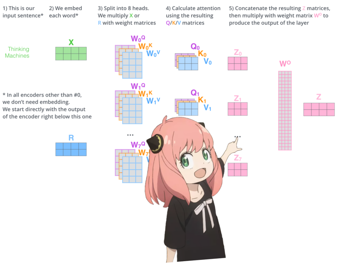
stacked_qkv_attention = torch.cat (qkv_attention_store, dim=-1) stacked_qkv_attention.shape
torch.Size ([17, 4096])
w_layer0 = model ["layers.0.attention.wo.weight"] w_layer0.shape
torch.Size ([4096, 4096])
embedding_delta = torch.matmul (stacked_qkv_attention, w_layer0.T) embedding_delta.shape
torch.Size ([17, 4096])
embedding_after_edit = token_embeddings_unnormalized + embedding_delta
embedding_after_edit.shape
torch.Size ([17, 4096])
embedding_after_edit_normalized = rms_norm (embedding_after_edit, model ["layers.0.ffn_norm.weight"]) embedding_after_edit_normalized.shape
torch.Size ([17, 4096])
w1 = model ["layers.0.feed_forward.w1.weight"] w2 = model ["layers.0.feed_forward.w2.weight"] w3 = model ["layers.0.feed_forward.w3.weight"] output_after_feedforward = torch.matmul (torch.functional.F.silu (torch.matmul (embedding_after_edit_normalized, w1.T)) * torch.matmul (embedding_after_edit_normalized, w3.T), w2.T) output_after_feedforward.shape
torch.Size ([17, 4096])
layer_0_embedding = embedding_after_edit+output_after_feedforward
layer_0_embedding.shape
torch.Size ([17, 4096])

final_embedding = token_embeddings_unnormalized
for layer in range (n_layers):
qkv_attention_store = []
layer_embedding_norm = rms_norm (final_embedding, model [f"layers.{layer}.attention_norm.weight"])
q_layer = model [f"layers.{layer}.attention.wq.weight"]
q_layer = q_layer.view (n_heads, q_layer.shape [0] //n_heads, dim)
k_layer = model [f"layers.{layer}.attention.wk.weight"]
k_layer = k_layer.view (n_kv_heads, k_layer.shape [0] //n_kv_heads, dim)
v_layer = model [f"layers.{layer}.attention.wv.weight"]
v_layer = v_layer.view (n_kv_heads, v_layer.shape [0] //n_kv_heads, dim)
w_layer = model [f"layers.{layer}.attention.wo.weight"]
for head in range (n_heads):
q_layer_head = q_layer [head]
k_layer_head = k_layer [head//4]
v_layer_head = v_layer [head//4]
q_per_token = torch.matmul (layer_embedding_norm, q_layer_head.T)
k_per_token = torch.matmul (layer_embedding_norm, k_layer_head.T)
v_per_token = torch.matmul (layer_embedding_norm, v_layer_head.T)
q_per_token_split_into_pairs = q_per_token.float ().view (q_per_token.shape [0], -1, 2)
q_per_token_as_complex_numbers = torch.view_as_complex (q_per_token_split_into_pairs)
q_per_token_split_into_pairs_rotated = torch.view_as_real (q_per_token_as_complex_numbers * freqs_cis)
q_per_token_rotated = q_per_token_split_into_pairs_rotated.view (q_per_token.shape)
k_per_token_split_into_pairs = k_per_token.float ().view (k_per_token.shape [0], -1, 2)
k_per_token_as_complex_numbers = torch.view_as_complex (k_per_token_split_into_pairs)
k_per_token_split_into_pairs_rotated = torch.view_as_real (k_per_token_as_complex_numbers * freqs_cis)
k_per_token_rotated = k_per_token_split_into_pairs_rotated.view (k_per_token.shape)
qk_per_token = torch.matmul (q_per_token_rotated, k_per_token_rotated.T)/(128)**0.5
mask = torch.full ((len (token_embeddings_unnormalized), len (token_embeddings_unnormalized)), float ("-inf"))
mask = torch.triu (mask, diagonal=1)
qk_per_token_after_masking = qk_per_token + mask
qk_per_token_after_masking_after_softmax = torch.nn.functional.softmax (qk_per_token_after_masking, dim=1).to (torch.bfloat16)
qkv_attention = torch.matmul (qk_per_token_after_masking_after_softmax, v_per_token)
qkv_attention_store.append (qkv_attention)
stacked_qkv_attention = torch.cat (qkv_attention_store, dim=-1)

w_layer = model [f"layers.{layer}.attention.wo.weight"]

embedding_delta = torch.matmul (stacked_qkv_attention, w_layer.T)

embedding_after_edit = final_embedding + embedding_delta

embedding_after_edit_normalized = rms_norm (embedding_after_edit, model [f"layers.{layer}.ffn_norm.weight"])

w1 = model [f"layers.{layer}.feed_forward.w1.weight"]

w2 = model [f"layers.{layer}.feed_forward.w2.weight"]

w3 = model [f"layers.{layer}.feed_forward.w3.weight"]

output_after_feedforward = torch.matmul (torch.functional.F.silu (torch.matmul (embedding_after_edit_normalized, w1.T)) * torch.matmul (embedding_after_edit_normalized, w3.T), w2.T)

final_embedding = embedding_after_edit+output_after_feedforward
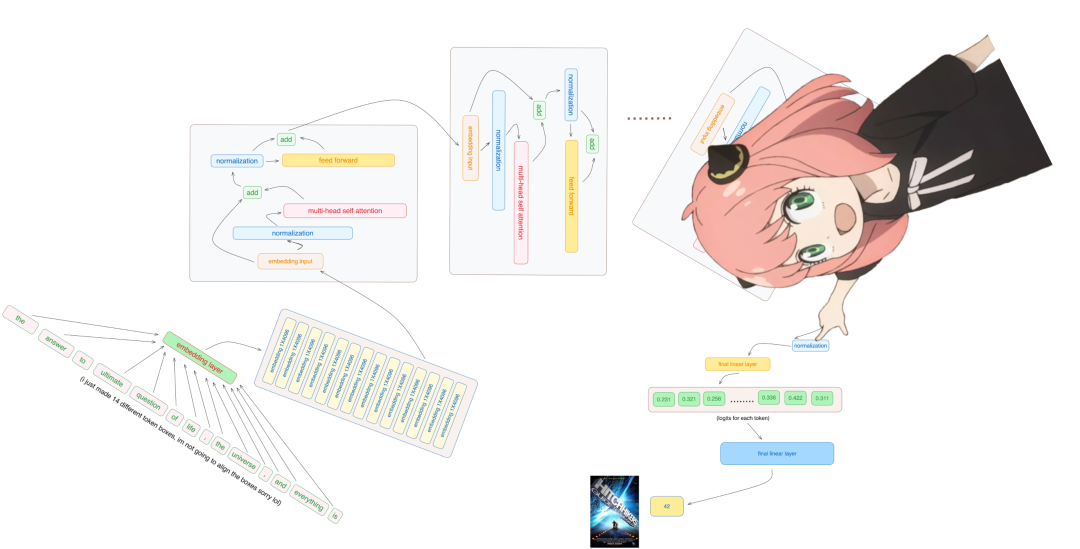
final_embedding = rms_norm (final_embedding, model ["norm.weight"]) final_embedding.shape
torch.Size ([17, 4096])
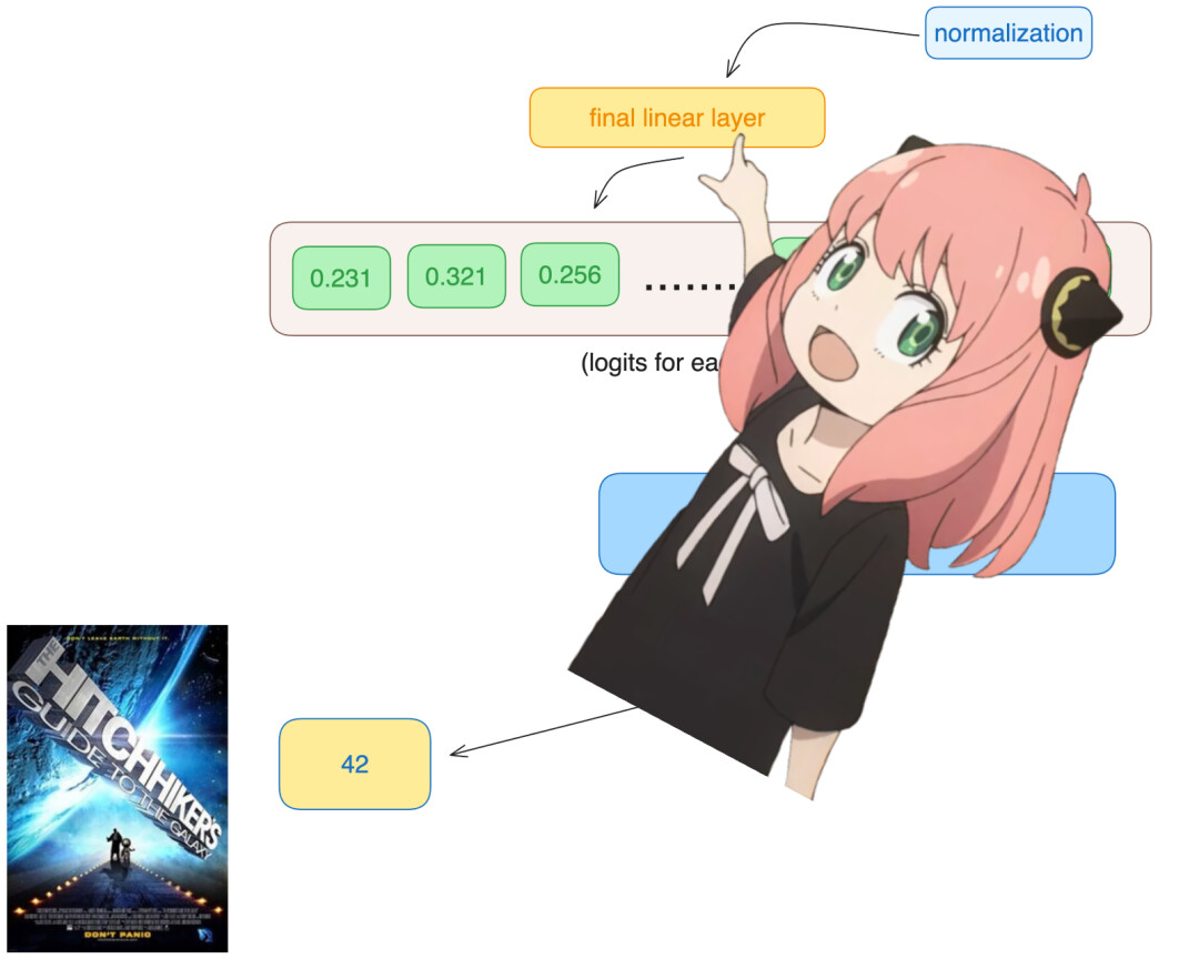
model ["output.weight"].shape
torch.Size ([128256, 4096])
logits = torch.matmul (final_embedding [-1], model ["output.weight"].T) logits.shape
torch.Size ([128256])
next_token = torch.argmax (logits, dim=-1) next_token
tensor (2983)

tokenizer.decode ([next_token.item ()])
'42'
整理不易,点赞三连↓